Algorithm Type and Hyperparameters
In this section, the range of values used will be indicated in blue.
Algorithm Type
PPO
There are several types of training algorithms:
- PPO: Uses policy learning, meaning it learns its value function from observations made by the current policy exploring the environment.
- SAC: Uses off-policy learning, meaning it can use observations made during the exploration of the environment by previous policies. However, SAC uses significantly more resources.
I started by using PPO algorithms as they are the default ones and SAC had library issues. However, after some modifications, I managed to use SAC algorithms.
Learning with SAC is very fast and works very well for simple actions. However, it is not possible to visually track the agent's progress given the resources required. I also observed poorer performance on complex learning tasks and a greater tendency to exploit any slight mechanical flaw.
Therefore, I switched back to PPO algorithms as they are more stable in learning, and I use SAC only to test a reward or a simple action to save time.
Hyperparameters
In reinforcement learning, hyperparameters are external settings to a machine learning model that influence the learning process. Unlike the internal parameters of a model, which are learned during training, hyperparameters must be set before training begins.
When using Unity ML-Agents to train intelligent agents, it is essential to understand and set the hyperparameters correctly to achieve good results. Here are some of the most important hyperparameters in Unity ML-Agents with the values I used for my model:
1. Learning Rate
1×10⁻⁴ - 3×10⁻⁴
The learning rate determines how quickly the model updates its internal parameters based on the errors observed during training. A too high learning rate can make learning unstable, while a too low rate can make it too slow. At the beginning of training, the agent starts with a learning rate of 0.0003 and ends with 0.0001. This value has a linear decay for each training session.
2. Batch Size
4096
Batch size is the number of data examples the model processes before updating its internal parameters. Larger batches can make learning more stable but require more memory. The value of 4096 seemed to be the best compromise between the necessary resources and the stability of learning.
3. Buffer Size
40960
Buffer size determines how many time steps are stored before the model updates its parameters. A larger buffer size can help stabilize learning but also increases memory requirements. A value of 40960 was used, which is twice the default value, reducing the number of agents trained simultaneously.
4. Gamma
0.995 - 0.998
Gamma is the discount factor, which determines the importance of future rewards relative to immediate rewards. A high gamma means the agent places more importance on future rewards. A value oscillating between 0.995 and 0.998 was used.
5. Lambda
0.95
Lambda is used in the calculation of the generalized advantage estimation (GAE) to control the bias-variance trade-off in advantage estimates. A higher lambda can reduce bias but increase variance. In our case, this value is 0.95, which is the default parameter.
6. Beta
0.001 - 0.005
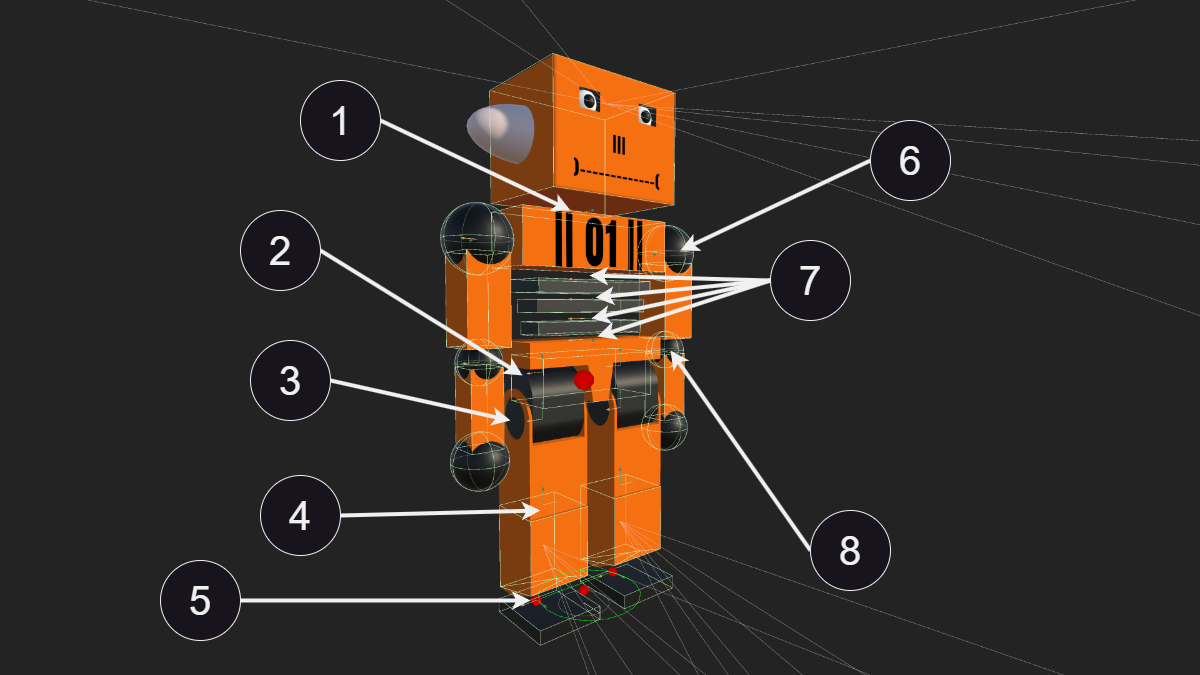
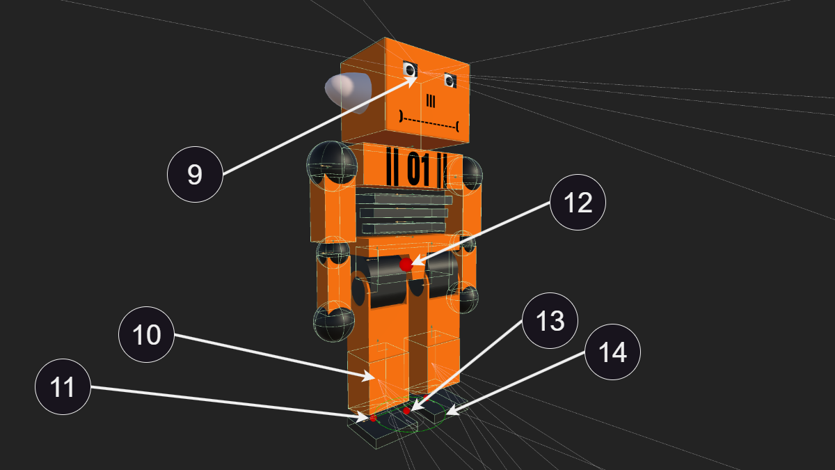
In policy algorithms, Beta is used for exploration. A high Beta promotes exploring new actions, while a low Beta favors exploiting known actions. A high Beta value (0.005) allows the agent to quickly learn to walk. However, keeping such a high value once the first steps are achieved is counterproductive. To be able to walk, the agent must perform a sequence of complex movements. If one of these movements is poorly executed, the agent loses balance and falls. If each of the 39 muscles has a too high percentage of performing a random action (discovery), it has little chance of achieving a movement that surpasses its previous record. Therefore, this value is set to 0.005 until the agent makes its first three steps, then it is set to 0.001. This value has a linear decay for each training session.
7. Epsilon
0.1 - 0.6
Epsilon is the acceptable threshold of divergence between the old and new policy during gradient descent updates. Setting this value to a low value will result in more stable updates but also slow down the training process. I found that a very high value (0.6) is necessary for the first steps and greatly accelerates learning, but this value must be lowered to 0.1 once the first steps are achieved. The problem with the first step is that the agent has little chance of achieving it randomly and only scores a few points before that. As with the Beta hyperparameter, the agent has little chance of making its first and second steps purely by chance. It is therefore preferable that it can quickly update its model once the first and second steps are achieved.
8. Num Layers
4
The number of layers in the neural network determines the depth of the model. Deeper networks can capture more complex relationships but are also more likely to overfit the training data. For my robot, I started training with 3 layers of 256 neurons. However, what seems to work best is 4 layers of 256 neurons with one layer having a dropout of 0.5. Dropout involves randomly disabling a fraction of the neurons during training and makes the model more robust by forcing it not to rely solely on one neural path. Adding dropout was initially to avoid overfitting, but I found that the agent learns much faster with it and maintains better stability.
Visualization of a neural model composed of 2 dense layers of 2 and 3 neurons respectively.
9. Hidden Units
256
This is the number of neurons per layer (Num layers). The number of hidden units per layer in the neural network affects the model's ability to learn complex representations from the input data. More hidden units increase modeling capacity but require more data and computation. Models tested with more than 256 neurons (512 and 1024) gave good results initially but quickly overfitted and took too long to train. With 128 neurons, the agent learns very quickly but is limited in the number of actions it can learn.
10. num_epoch
3 - 6
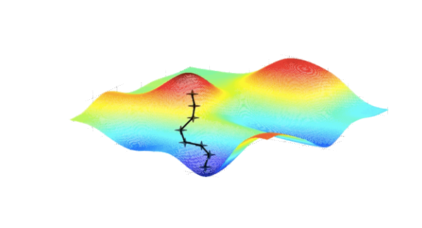
num_epoch is the number of passes through the experience buffer during gradient descent. Lowering this value will ensure more stable updates at the cost of slower training. I use a value of 3 for normal training and 6 when I need to run tests and only training time matters.
Visualization of gradient descent, a commonly used optimization algorithm in machine learning and reinforcement learning.
11. Activation Function
ReLu
Normally, Unity does not offer to modify the activation function and uses the ReLu function (f(x)=max(0,x)).
ReLU (Rectified Linear Unit) f(x) = max(0, x)
ReLU is a simple and effective function, defined as the maximum between 0 and the input x. It helps mitigate the issues of exploding or vanishing gradients and introduces sparsity in the network, which can improve model efficiency.
Swish f(x) = x · sigmoid(x)
Swish is defined as the product of the input x and the sigmoid function of x. Swish is a smooth function, offering more stable gradients and can improve performance and convergence speed in certain learning contexts.
Advantages of Swish
- Smoothness: Provides more stable gradients.
- Performance: Can offer better performance than ReLU in some applications.
- Flexibility: Better flexibility in learning complex relationships in the data.
Due to lack of time, I did not implement the Swish function (f(x)=x⋅sigmoid(x)) in the final version. However, I tested this function which seems to give good results and will likely pursue this direction in the future.


